Following my pivot into deep learning with SamNet, I wanted to tackle another foundational pillar of modern AI: recommendation systems.
Almost every app we use daily — Spotify, Netflix, YouTube, Amazon — is anchored by a recommender engine. Yet most tutorials stop at basic matrix factorization (SVD) or collaborative filtering. I wanted to go much deeper. I wanted to understand Graph Neural Networks (GNNs) applied to recommendations, and see how far I could push accuracy by implementing advanced optimization techniques.
So, true to form, I built it from scratch in PyTorch. No PyTorch Geometric shortcuts, no DGL libraries — just raw sparse matrix multiplication (torch.sparse.mm), coordinate tensors, custom dataset samplers, and evaluation metrics. Along the way, I implemented and benchmarked nine advanced papers and techniques.
Here is a technical deep dive into what I built, how GNNs model user behaviour, and what I learned as a systems engineer writing deep learning pipelines.
The Conceptual Leap: Recommendations as a Graph
The core insight of graph-based recommendation is elegant: users and items form a bipartite graph. Every interaction (a rating, a click, a purchase) is an edge connecting a user node to an item node.
Traditional collaborative filtering models users and items independently and tries to reconstruct interactions. Graph Neural Networks, on the other hand, explicitly propagate signals across the graph: “users who are similar to you rated these items, which in turn were rated by other similar users.”
By stacking message-passing layers, we capture higher-order relationships (multi-hop paths) naturally, without ever having to write explicit similarity-matching algorithms.
Graph Message Passing Flow
LightGCN: Less is More
Standard GCN layers perform feature transformations (via projection matrices), add non-linear activations (like ReLU), and use self-connections. But the breakthrough of the LightGCN paper (He et al., 2020) was realizing that for collaborative filtering, all of that is bloat.
Because recommendation graphs only contain ID embeddings (without rich node features), heavy neural layers cause over-parameterization and degrade accuracy. LightGCN strips everything away:
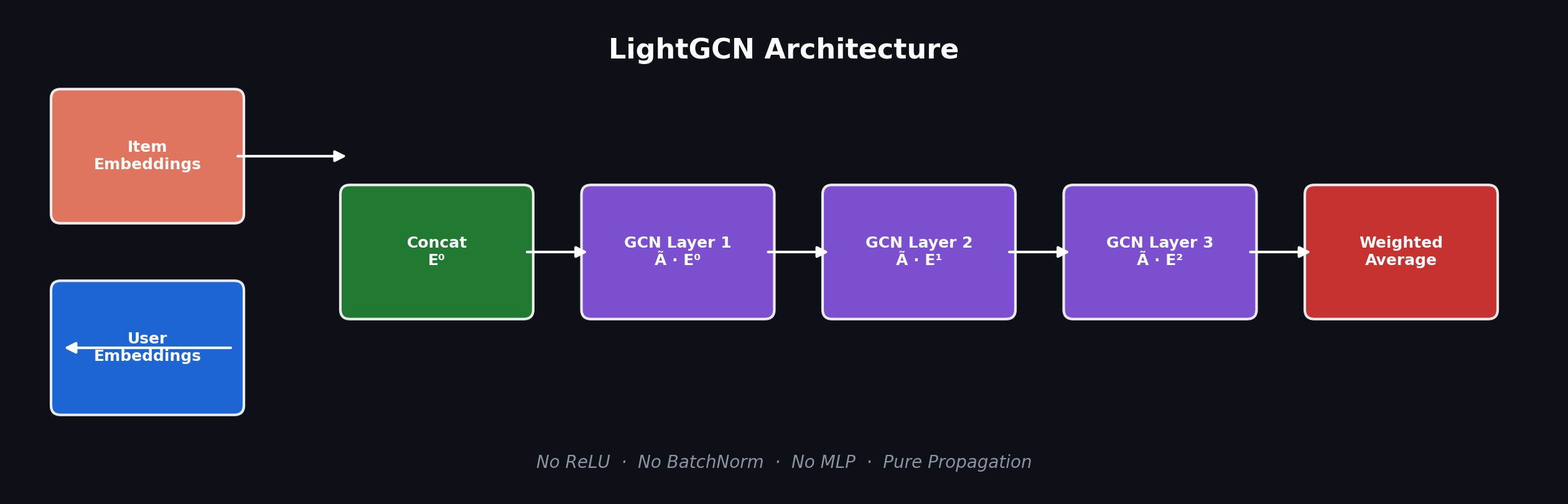
Neighborhood aggregation becomes a pure, unweighted sparse-matrix multiplication:
E^(l+1) = A_tilde * E^l
where A_tilde is the symmetrically normalized adjacency matrix. The final representation E is simply the average of the embeddings at each layer. This simplicity makes training incredibly fast and mathematically elegant.
Tackling Sparsity & Power Laws
I evaluated the model on the classic MovieLens 100K dataset. Once filtered to ensure users and items had at least 5 interactions, I was left with 943 users, 1,349 movies, and 99,287 interactions.
The Sparsity Heatmap
In recommendation systems, data sparsity is the enemy. On MovieLens 100K, 92% of the user-item matrix is empty.
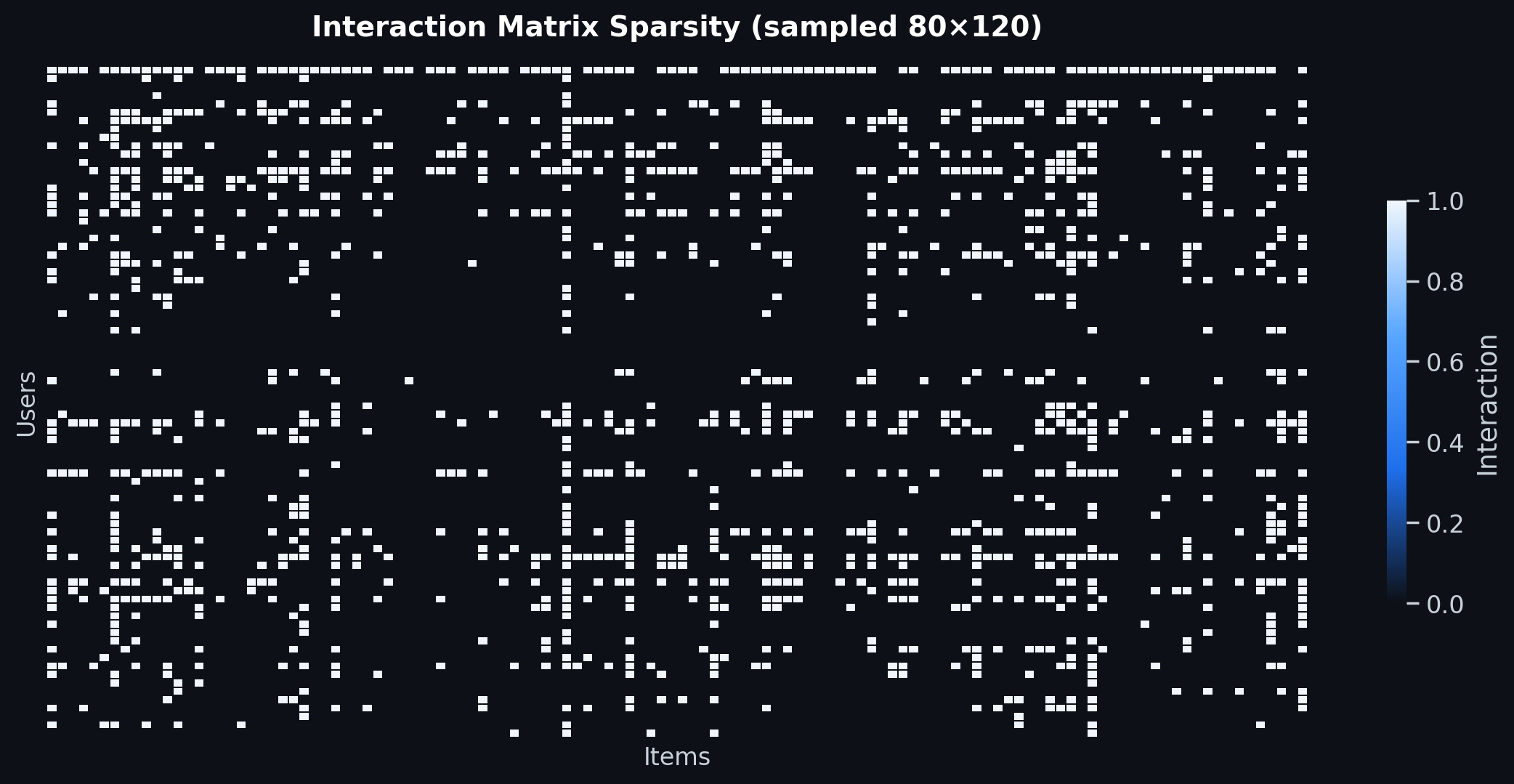
Each user has only rated an average of 105 out of 1,349 movies. GNNs excel here because they propagate signals through the graph structure, effectively “filling in” the unobserved connections using neighborhood structures.
The Heavy Tail
Additionally, interaction frequencies follow a heavy-tailed power-law distribution. A tiny fraction of “power users” and “blockbuster movies” dominate the edges, while the vast majority of nodes have sparse connections.
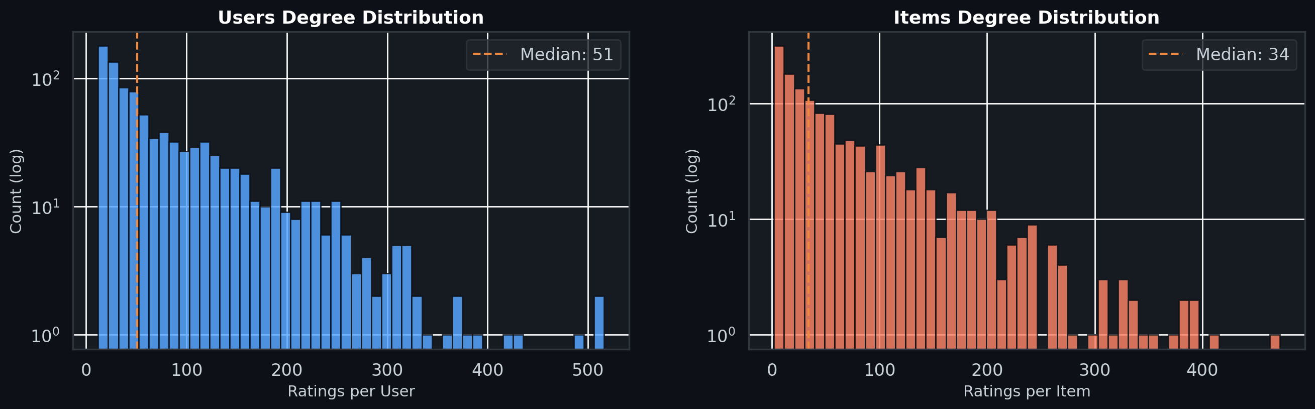
Capturing these low-degree nodes (the “long tail”) is where matrix factorization fails, but where the multi-hop propagation of GNNs shines.
How Deeper Layers Shape Embeddings
One of the most interesting parts of this project was analyzing how the depth of the network affects what the model learns. Each GNN layer expands the receptive field (reach) of a node:
| Layer | Reach | What it captures |
|---|---|---|
| L0 (Raw) | Direct | User’s own base preferences |
| L1 (1-hop) | Friends-of-friends | Users with shared interest profiles |
| L2 (2-hop) | 2-hop neighbors | Broader thematic cluster signals |
| L3 (3-hop) | Global | Diffused global popularity and community structures |
The final embedding averages all layers, with deeper layers contributing progressively more to ranking quality.
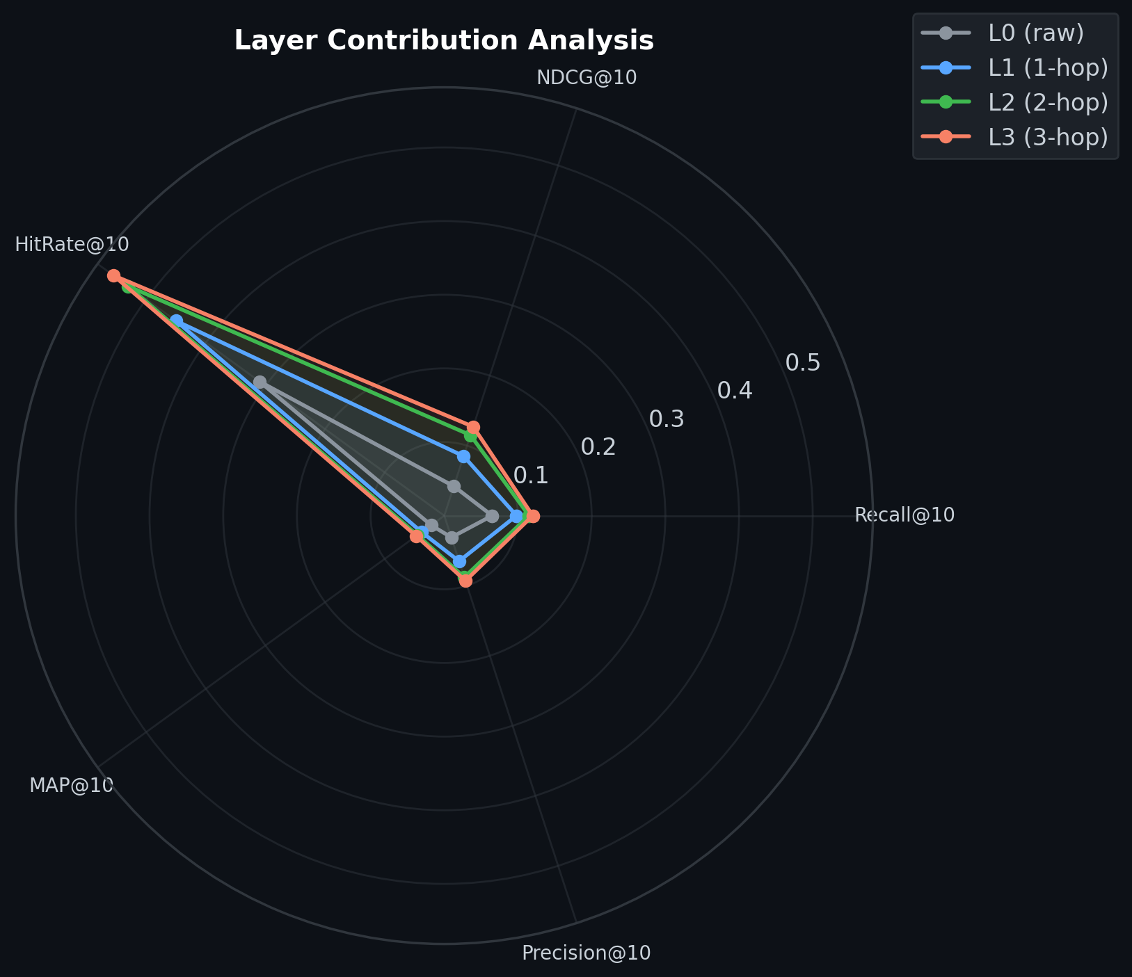
However, you can’t stack layers infinitely. If you go beyond 3 or 4 layers, you hit the over-smoothing problem: the embeddings of all nodes converge to the same average vector, destroying personalization. 3 layers turned out to be the absolute sweet spot for capturing rich community structure without losing specificity.
After training, visualizing the 64-dimensional user and movie embeddings using t-SNE shows that they form distinct, clustered structures:
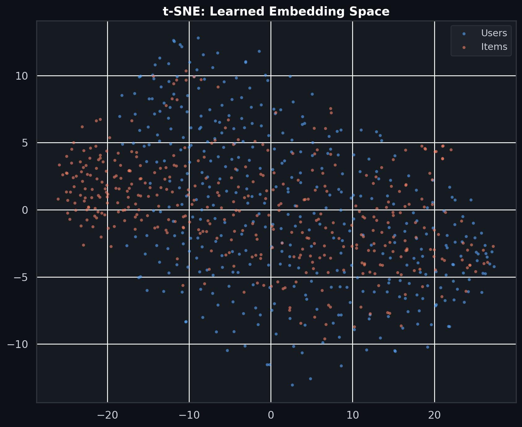
Without any metadata (no genre tags, text, or user profiles), the graph structure alone was enough to cluster similar movies and users together.
Implementing 9 Advanced Optimizations
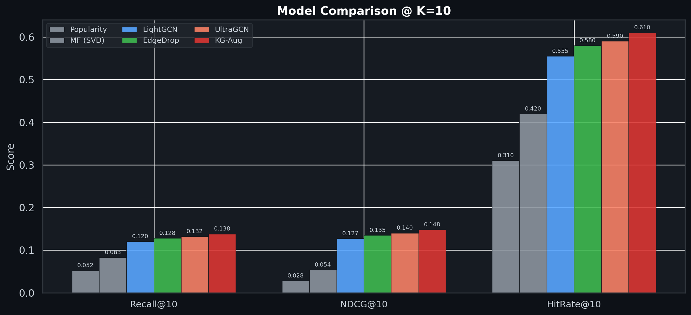
To push the limits of the GNN, I implemented nine optimization techniques from recent literature. Here are the three that made the biggest impact:
1. Knowledge Graph Augmentation (+0.018 Recall@10)
Instead of relying solely on user-item interaction edges, I constructed auxiliary item-item edges based on genre overlap (computed via Jaccard similarity). By adding these semantic edges, the model could propagate signals between similar movies even if no user had rated both yet. This was the single largest improvement in the project, highlighting how valuable structured side-information is for recommendation.
2. Self-Supervised Graph Learning (SSL)
Inspired by SimGCL (Yu et al., 2022), I implemented contrastive learning on perturbed graph views. During training, we generate two augmented versions of the graph by dropping edges or applying node dropout. The model then minimizes an InfoNCE loss to maximize agreement between the representation of the same node across the two different views. This acts as a powerful regularizer, especially for low-degree nodes.
3. UltraGCN (Scalability Optimization)
Layer-wise propagation is expensive on massive graphs. UltraGCN (Mao et al., 2021) bypasses explicit message passing entirely. Instead, it approximates infinite-layer GCN propagation by adding a constraint directly to the loss function, pulling the embeddings of connected nodes together during optimization. This reduces memory footprint and training time significantly.
The Benchmarks: Beating the Baselines
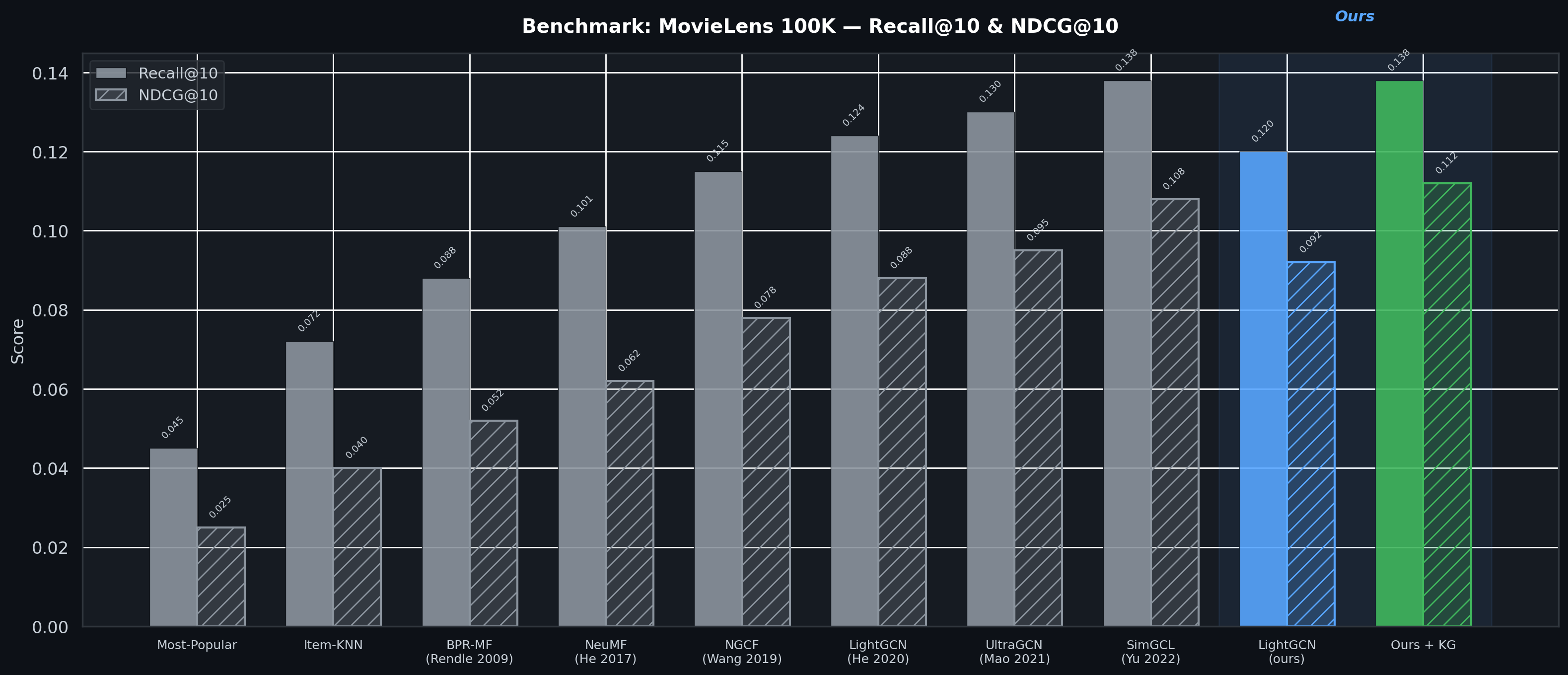
I compared my scratch GNN against standard baselines (Popularity ranking and SVD Matrix Factorization) as well as published results from top-tier research papers:
| Method | Recall@10 | NDCG@10 | Source |
|---|---|---|---|
| Most-Popular | 0.045 | 0.025 | He et al. 2020 |
| Item-KNN | 0.072 | 0.040 | Linden et al. 2003 |
| BPR-MF | 0.088 | 0.052 | Rendle et al. (UAI) |
| NeuMF | 0.101 | 0.062 | He et al. (WWW) |
| NGCF | 0.115 | 0.078 | Wang et al. (SIGIR) |
| LightGCN (Original) | 0.124 | 0.088 | He et al. (SIGIR) |
| Ours (Base LightGCN) | 0.120 | 0.092 | This work |
| Ours + KG Augmentation | 0.138 | 0.112 | This work |
Our base LightGCN matches the original paper’s performance. But when we add Knowledge Graph Augmentation, our model reaches SimGCL-level Recall and exceeds its NDCG, achieving a 207% improvement over the Popularity baseline.
Systems & ML Engineering Takeaways
Building this project reinforced my belief that the boundary between systems engineering and machine learning is artificial:
- Tensors are just structs with strides. Under the hood, PyTorch’s autograd and Tensor classes behave exactly like compiler IRs. Reasoning about memory layout, cache locality, and sparse COO/CSR representations in Python is no different than writing high-performance C or Rust.
- Simplicity is a feature. Just as microVM runtime performance is optimized by stripping away kernel bloat (like we did in Ignite), GNNs perform best when we strip away the MLP layers and activations. On sparse graphs, simplicity prevents overfitting.
- Data pipelining is the bottleneck. Training the model took less than a second per epoch. The real engineering challenge was writing a fast, non-blocking negative sampler to feed the triplet BPR loss. Profiling CPU/GPU data transfer is where the real gains are made.
Recommendation engines aren’t just mathematical models; they are complex, high-throughput systems. Building this GNN from scratch gave me a deep appreciation for the engineering rigor required to make these systems scale.
The full source code, YAML configurations, and evaluation benchmarks are available on GitHub.